Manual¶

Table of contents

This manual provides reference documentation to PETGEM from a user’s and developer’s perspective.

How generate documentation ¶

PETGEM is documented in PDF and HTML format using Sphinx and LaTeX. The documentation source is in the doc/ directory. The following steps summarize how to generate PETGEM documentation.

Move to the PETGEM doc directory:
```
$ cd doc
```
Generate the PETGEM documentation in HTML format by typing:
```
$ make html
```
Or, if you prefer the PDF format by typing:
```
$ make latexpdf
```
The previous steps will build the documentation in the doc/build directory. Alternatively, you can modify this path by editing the file setup.cfg and provide the required information below [build_sphinx] section:
```
[build_sphinx]
source-dir = doc/source
build-dir  = usr/local/path-build
all_files  = 1
```

Coding style ¶

PETGEM’s coding style is based on PEP-0008 guidelines. Main guidelines are the following:

79 characteres per line.
4 spaces per indentation level.
Variables are lower case meanwhile constants are upper case.

Comments convention for functions is as follows:

def function(arg1, arg2):
    ''' This is a function.

        :param int arg1: array of dimensions ...
        :param str arg2: string that ...
    '''

The use of inline comments is sparingly.
Use of lowercase to name functions. Furthermore, functions names have following form: <actionSubject>(), e.g. computeMatrix().
Use of whole words instead abbreviations, examples:
- Yes: solveSystem(), computeEdges(), computeMatrix().
- No: solve(), compEdges(), compMatrix().

PETGEM use a code structure for the high-order Nédelec FE algorithm that emphasizes good parallel scalability, which is crucial in the multi-core era. Furthermore, it’s modularity should simplify the process of reaching the best possible performance in terms of percentage of the peak amount of floating point operations provided by the architecture. The code structure is modular, simple and flexible which allows exploiting not just PETGEM modules but also third party libraries. Therefore, the software stack includes interfaces to external suites of data structures and libraries that contain most of the necessary building blocks needed for programming large scale numerical applications, i.e. sparse matrices, vectors, iterative and direct solvers. As a result, the code is compact and flexible whose main UML diagrams are described as follows.

PETGEM directory structure ¶

This subsection is dedicated to list and describe the PETGEM directory structure.

Top directory structure¶
Name	Description
doc/	Source files for PETGEM documentation
examples/	Templates of basic scripts for 3D CSEM/MT modelling
petgem/	Source code
kernel.py	Heart of the code. This file contains the entire work-flow for a 3D CSEM/MT survey
DESCRIPTION.rst	Summary of PETGEM features, requirements and installation instructions
LICENSE.rst	License file
MANIFEST.in	File with exact list of files to include in PETGEM distribution
README.rst	Readme file
setup.py	Main PETGEM setup script, it is based on Python setup-module
setup.cfg	Setup configuration file for PETGEM setup script

The PETGEM source code is petgem/, which has the following contents:

petgem/ directory structure¶
Name	Description
common.py	Common classes and functions for init process.
hvfem.py	General modules and classes for describing a 3D CSEM/MT survey by using HEFEM ( $p=1,2,3,4,5,6$ ) in tetrahedral meshes
mesh.py	Interface to import mesh files
parallel.py	Modules for supporting parallel computations and solution of 3D CSEM/MT
preprocessing.py	Modules for PETGEM pre-processing
solver.py	Parallel functions within PETGEM and interface to PETSc solvers

Running a simulation ¶

This section introduces the basics of running PETGEM on the command line. In order to solve a 3D CSEM/MT survey, the PETGEM kernel requires two files, namely, the petsc.opts file and the params.yaml file, which are described below.

Options for PETSc solvers/preconditioners are accessible via the petsc.opts file, a glance of this is the following:

# Solver options for PETSc
-ksp_type gmres
-pc_type sor
-ksp_rtol 1e-8
-ksp_converged_reason
-ksp_monitor

Please, see PETSc documentation for more details about available options. A template of this file is included in examples/ of the PETGEM source tree. Additionally, a freely available copy of this file is located at Download section.

On the other hand, any 3D CSEM/MT survey should include: order for Nédélec elements discretizations, physical parameters, a mesh file, source and receivers files. These data are included in the params.yaml file. In order to avoid a specific parser, params.yaml file is imported by PETGEM as a Python dictionary. As consequence, the dictionary name and his key names MUST NOT BE changed.

A glance of params.yaml file is the following:

###############################################################################
# PETGEM parameters file
###############################################################################
# Model parameters
model:
  mode: mt    # Modeling mode: csem or mt
  csem:
    sigma:
      #file: 'my_file.h5'                # Conductivity model file
      horizontal: [1.e-10, 0.01]       # Horizontal conductivity
      vertical: [1.e-10, 0.01]         # Vertical conductivity
    source:
      frequency: 2.                     # Frequency (Hz)
      position: [1750., 1750., -975.]   # Source position (xyz)
      azimuth: 0.                       # Source rotation in xy plane (in degrees)
      dip: 0.                           # Source rotation in xz plane (in degrees)
      current: 1.                       # Source current (Am)
      length: 1.                        # Source length  (m)
  mt:
    sigma:
      #file: 'my_file.h5'                # Conductivity model file
      horizontal: [1.e-10, 0.01]       # Horizontal conductivity
      vertical: [1.e-10, 0.01]         # Vertical conductivity
    frequency: 2.                      # Frequency (Hz)
    polarization: 'xy'                 # Polarization mode for mt (xyz)

  # Common parameters for all models
  mesh: examples/case_MT/mesh_trapezoidal.msh   # Mesh file (gmsh format v2)
  receivers: examples/case_MT/receivers.h5 # Receiver positions file (xyz)

# Execution parameters
run:
  nord: 1       # Vector basis order (1,2,3,4,5,6)
  cuda: False   # Cuda support (True or False)

# Output parameters
output:
  vtk: False                               # Postprocess vtk file (EM fields, conductivity)
  directory: examples/case_MT/out           # Directory for output (results)
  directory_scratch: examples/case_MT/tmp   # Directory for temporal files

The params.yaml file is divided into 3 sections, namely, model, run and output.

A template of params.yaml file is included in examples/ of the PETGEM source tree. Additionally, a freely available copy of this file is located at Download section.

Once the petsc.opts file and the params.yaml file are ready, the PETGEM kernel is invoked as follows:

$ mpirun -n MPI_tasks python3 kernel.py -options_file path/petsc.opts path/params.yaml

where MPI_tasks is the number of MPI parallel tasks, kernel.py is the script that manages the PETGEM work-flow, petsc.opts is the PETSc options file and params.yaml is the modelling parameters file for PETGEM.

PETGEM solves the problem and outputs the solution to the output.directory/ path. The output file will be in h5py format. By default, the file structure contains a fields dataset and a receiver_coordinates dataset. In example, if the model has 3 receivers, fields dataset would contain six components (Ex, Ey, Ez, Hx, Hy, Hz) of the electromagnetic field responses as follows (fields only for illustrative purposes):

      Ex-component               Ey-component              Ez-component                 Hx-component             Hy-component              Hz-component
-4.5574e-13+7.1233e-13j       4.6739e-14+2.5366e-14j    -3.1475e-13+3.7062e-13j     -4.5574e-13+7.1233e-13j   4.6739e-14+2.5366e-14j    -3.1475e-13+3.7062e-13j
-6.3279e-13+7.1644e-13j       9.0092e-14+5.6392e-14j    -5.3662e-13+3.7808e-13j     -6.3279e-13+7.1644e-13j   9.0092e-14+5.6392e-14j    -5.3662e-13+3.7808e-13j
-1.0010e-12+7.0402e-13j       1.0689e-13+3.6703e-14j    -7.8662e-13+3.6350e-13j     -1.0010e-12+7.0402e-13j   1.0689e-13+3.6703e-14j    -7.8662e-13+3.6350e-13j

It is worth to mention the fields will be separated by real and imaginary component.On the other hand, the receiver coordinates as follows (receiver_coordinates):

  X         Y                   Z
         1750.    -990
         1750.    -990
         1750.    -990

In summary, for a general 3D CSEM/MT survey, the kernel.py script follows the next work-flow:

kernel.py reads a params.yaml
Following the contents of the params.yaml, a problem instance is created
Runs the data preprocessing
The problem sets up its domain, sub-domains, source-type, solver. This stage include the computation of the main data structures
Parallel assembling of $Ax=b$ .
The solution is obtained in parallel by calling a ksp() PETSc object.
Interpolation of electromagnetic (electric and magnetic) responses and post-processing parallel stage
Finally the solution can be stored by calling solver.postprocess() method. Current version support h5py format.

Based on previous work-flow, any 3D CSEM/MT modelling requires the following input files:

A mesh file (current version supports mesh files from Gmsh)
A conductivity model associated with the materials defined in the mesh file
A list of receivers positions in hdf5 format for the electric responses post-processing
A params.yaml file where are defined the 3D CSEM/MT parameters
A petsc.opts file where are defined options for PETSc solvers

During the preprocessing stage, the kernel.py generates the mesh file (Gmsh format) with its conductivity model and receivers positions in PETSc binary files.

For this phase, the supported/expected formats are the following:

basis_order: nédélec basis element order for the discretization. Supported orders are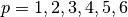 $p=1,2,3,4,5,6$
mesh_file: path to tetrahedral mesh file in format from Gmsh
sigma: numpy array or hdf5 file where each value represents the horizontal and vertical conductivity for each material defined in mesh_file. Therefore, size of sigma must match with the number of materials in mesh_file
receivers_file: floating point values giving the X, Y and Z coordinates of each receiver in hdf5 format. Therefore, the number of receivers in the modelling will defined the number of the rows in receivers_file, i.e. if the modelling has 3 receivers, receivers_file should be:
```
5.8333300e+01   1.7500000e+03  -9.9000000e+02
1.1666670e+02   1.7500000e+03  -9.9000000e+02
1.7500000e+02   1.7500000e+03  -9.9000000e+02
```
output_directory_scratch: output scratch directory for pre-processing task

Once the previous information has been provided, the kernel.py script will generate all the input files required by PETGEM in order to solve a 3D CSEM/MT survey. The kernel.py output files list is the following:

nodes.dat: floating point values giving the X, Y and Z coordinates of the four nodes that make up each tetrahedral element in the mesh. The dimensions of nodes.dat are given by (number-of-elements, 12)
meshConnectivity.dat: list of the node number of the n-th tetrahedral element in the mesh. The dimensions of meshConnectivity.dat are given by (number-of-elements, 4)
dofs.dat: list of degrees of freedom of the n-th tetrahedral element in the mesh. Since PETGEM is based on high-order Nédelec FE, the dimensions of dofs.dat are given by (number-of-elements, 6) for $p=1$ , by (number-of-elements, 20) for $p=2$ , by (number-of-elements, 45) for $p=3$ , by (number-of-elements, 84) for $p=4$ , by (number-of-elements, 140) for $p=5$ , and by (number-of-elements, 216) for $p=6$ .
edges.dat: list of the edges number of the n-th tetrahedral element in the mesh. The dimensions of edges.dat are given by (number-of-elements, 6)
faces.dat: list of the faces number of the n-th tetrahedral element in the mesh. The dimensions of faces.dat are given by (number-of-elements, 4)
edgesNodes.dat: list of the two nodes that make up each edge in the mesh. The dimensions of edgesNodes.dat are given by (number-of-edges, 2)
faces.dat: list of the four faces that make up each tetrahedral element in the mesh. The dimensions of faces.dat are given by (number-of-elements, 4)
facesNodes.dat: list of the three nodes that make up each tetrahedral face in the mesh. The dimensions of facesNodes.dat are given by (number-of-faces, 3)
boundaries.dat: list of the DOFs indexes that belongs on domain boundaries. The dimensions of boundaries.dat are given by (number-of-boundaries, 1)
conductivityModel.dat: floating point values giving the conductivity to which the n-th tetrahedral element belongs. The dimensions of conductivityModel.dat are given by (number-of-elements, 1)
receivers.dat: floating point values giving the X, Y and Z coordinates of the receivers. Additionally, this file includes information about the tetrahedral element that contains the n-th receiver, namely, its X, Y and Z coordinates of the four nodes, its list of the node number and its list of DOFs.
nnz.dat: list containing the number of nonzeros in the various matrix rows, namely, the sparsity pattern. According to the PETSc documentation, using the nnz.dat list to preallocate memory is especially important for efficient matrix assembly if the number of nonzeros varies considerably among the rows. The dimensions of nnz.dat are given by (number-of-DOFs, 1)

For each *.dat output file, the kernel.py script will generate *.info files which are PETSc control information.

For post-processing stage (interpolation of electric responses at receivers positions) a point location function is needed. For this task, PETGEM is based on find_simplex function by Scipy, which find the tetrahedral elements (simplices) containing the given receivers points. If some receivers positions are not found, PETGEM will print its indexes and will save only those located points in the receivers.dat file.

Mesh formats ¶

Current PETGEM version supports mesh files from Gmsh. Aforementioned format must be pre-processed using the run_preprocessing.py script. The run_preprocessing.py script is included in the top-level directory of the PETGEM source tree.

Available solvers ¶

This section describes solvers available in PETGEM from an user’s perspective. Direct as well as iterative solvers and preconditioners are supported through an interface to PETSc library.

PETGEM uses petsc4py package in order to support the Krylov Subspace Package (KSP) from PETSc. The object KSP provides an easy-to-use interface to the combination of a parallel Krylov iterative method and a preconditioner (PC) or a sequential/parallel direct solver. As result, PETGEM users can set various solver options and preconditioner options at runtime via the PETSc options database. These parameters are defined in the petsc.opts file.

Simulations in parallel ¶

In FEM or HEFEM simulations, the need for efficient algorithms for assembling the matrices may be crucial, especially when the DOFs is considerably large. This is the case for realistic scenarios of 3D CSEM surveys because the required accuracy. In such situation, assembly process remains a critical portion of the code optimization since solution of linear systems which asymptotically dominates in large-scale computing, could be done with linear solvers such as PETSc, MUMPs, PARDISO). In fact, in PETGEM V0.6, the system assembly takes around $15%$ of the total time.

The classical assembly in FEM or HEFEM programming is based on a loop over the elements. Different techniques and algorithms have been proposed and nowadays is possible performing these computations at the same time, i.e., to compute them in parallel. However, parallel programming is not a trivial task in most programming languages, and demands a strong theoretical knowledge about the hardware architecture. Fortunately, Python presents user friendly solutions for parallel computations, namely, mpi4py and petsc4py . These open-source packages provides bindings of the MPI standard and the PETSc library for the Python programming language, allowing any Python code to exploit multiple processors architectures.

On top of that, Figure 7.4 depicts shows an upper view of the matrix assembly and solution using the mpi4py and petsc4py package in PETGEM. The first step is to partition the work-load into subdomains. This task can be done by PETSc library, which makes load over processes balanced. After domain partition, subdomains are assigned to MPI tasks and the elemental matrices are calculated concurrently. These local contributions are then accumulated into the global matrix system. The process for global vector assembly is similar.

Subsequently, the system is ready to be solved. PETGEM uses the Krylov Subspace Package (KSP) from PETSc through the petsc4py package. The KSP object provides an easy-to-use interface to the combination of a parallel Krylov iterative method and a preconditioner (PC) or a sequential/parallel direct solver. As result, PETGEM users can set various solver options and preconditioner options at runtime via the PETSc options database. Since PETSc knows which portions of the matrix and vectors are locally owned by each processor, the post-processing task is also completed in parallel.

All petsc4py classes and methods are called from the PETGEM kernel in a manner that allows a parallel matrix and parallel vectors to be created automatically when the code is run on many processors. Similarly, if only one processor is specified the code will run in a sequential mode. Although petsc4py allows control the way in which the matrices and vectors to be split across the processors on the architecture, PETGEM simply let petsc4py decide the local sizes in sake of computational flexibility. However, this can be modified in an easy way without any extra coding required.

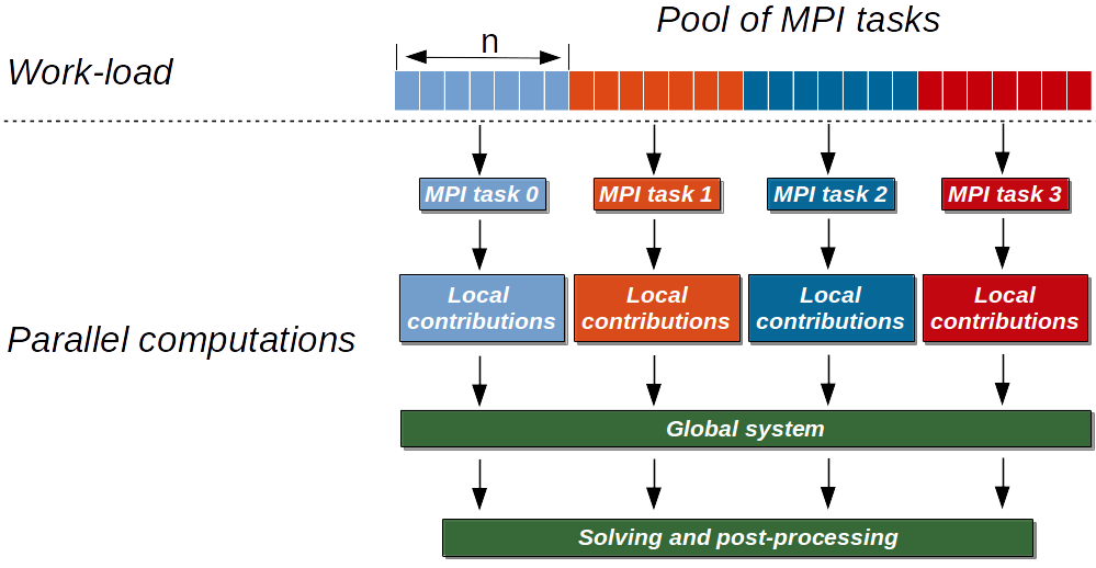
Parallel scheme for assembly in PETGEM V1.0.0

Figure 7.4. Parallel scheme for assembly and solution in PETGEM using 4 MPI tasks. Here the elemental matrices computation is done in parallel. After calculations the global system is built and solved in parallel using the petsc4py and mpi4py packages.¶

Visualization of results ¶

Once a solution of a 3D CSEM/MT survey has been obtained, it should be post-processed by using a visualization program. PETGEM does not do the visualization by itself, but it generates output files (hdf5 and VTK are supported) with the electric responses at receivers positions and nodes in the mesh. It also gives timing values in order to evaluate the performance.

Figure 7.5 shows an example of PETGEM output for the first modelling case (Canonical model of an off-shore hydrocarbon reservoir) described in CSEM example section. Figure 7.5 was obtained using Paraview.

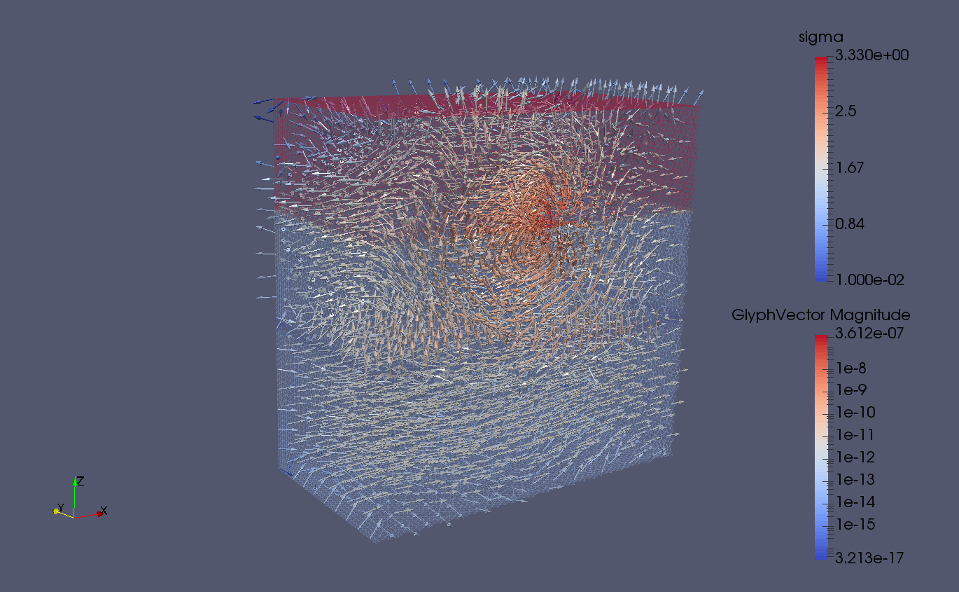
Figure 7.5. PETGEM vtk output.¶

CSEM example ¶

This section includes a step-by-step walk-through of the process to solve a simple 3D CSEM survey. The typical process to solve a problem using PETGEM is followed: a model is meshed, PETGEM input files are preprocessed and modeled by using kernel.py script to solve the modelling and finally the results of the simulation are visualised.

All necessary data to reproduce the following examples are available in the Download section.

Example 1: Canonical model of an off-shore hydrocarbon reservoir ¶

Model ¶

In order to explain the 3D CSEM modelling using PETGEM, here is considered the canonical model by Weiss2006 which consists in four-layers: 1000 m thick seawater (3.3 $S/m$ ), 1000 m thick sediments (1 $S/m$ ), 100 m thick oil (0.01 $S/m$ ) and 1400 m thick sediments (1 $S/m$ ). The computational domain is a $[0,3500]^3$ m cube. For this model, a 2 Hz x-directed dipole source is located at $z=975$ , $x=1750$ , $y=1750$ . The receivers are placed in-line to the source position and along its orientation, directly above the seafloor ( $z = 990$ ). Further, the Nédélec element order is p=1 (first order)

Meshing ¶

PETGEM V1.0 is based on tetrahedral meshes. Therefore, Figure 7.8 shows a 3D view of the model with its unstructured tetrahedral mesh for the halfspace $y>1750$ , with the color scale representing the electrical conductivity $\sigma$ for each layer. Mesh in Figure 7.8 have been obtained using Gmsh.

In-line canonical off-shore hydrocarbon model with its unstructured tetrahedral mesh for :math:`y>150`

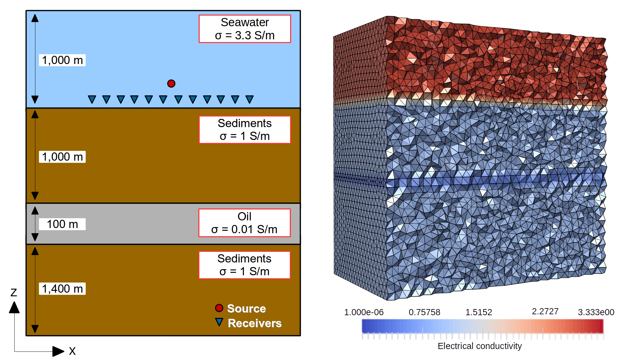
Figure 7.8. In-line canonical off-shore hydrocarbon model with its unstructured tetrahedral mesh for $y>1750$ . The color scale represents the electrical conductivity $\sigma$ for each layer.¶

In this case, the mesh is composed by four conductivity materials. Please, see Gmsh manual for details about the mesh creation process.

Parameters file for PETGEM ¶

The parameters file used for this example follows:

###############################################################################
# PETGEM parameters file
###############################################################################
# Model parameters
model:
  mode: csem    # Modeling mode: csem or mt
  csem:
    sigma:
      #file: 'my_file.h5'                # Conductivity model file
      horizontal: [1., 0.01, 1., 3.3333]  # Horizontal conductivity
      vertical: [1., 0.01, 1., 3.3333]    # Vertical conductivity
    source:
      frequency: 2.                     # Frequency (Hz)
      position: [1750., 1750., -975.]   # Source position (xyz)
      azimuth: 0.                       # Source rotation in xy plane (in degrees)
      dip: 0.                           # Source rotation in xz plane (in degrees)
      current: 1.                       # Source current (Am)
      length: 1.                        # Source length  (m)

  # Common parameters for all models
  mesh: examples/case_1/DIPOLE1D.msh   # Mesh file (gmsh format v2)
  receivers: examples/case_1/receiver_pos.h5 # Receiver positions file (xyz)

# Execution parameters
run:
  nord: 1       # Vector basis order (1,2,3,4,5,6)
  cuda: False   # Cuda support (True or False)

# Output parameters
output:
  vtk: True                               # Postprocess vtk file (EM fields, conductivity)
  directory: examples/case_1/out           # Directory for output (results)
  directory_scratch: examples/case_1/tmp   # Directory for temporal files

Note that you may wish to change the location of the input files to somewhere on your drive. The solver options have been configured in the petsc.opts file as follows:

# Solver options for
-ksp_type gmres
-pc_type sor
-ksp_rtol 1e-8
-ksp_converged_reason
-log_summary

That’s it, we are now ready to solve the modelling.

Running PETGEM ¶

To run the simulation, the following command should be run in the top-level directory of the PETGEM source tree:

$ mpirun -n 16 python3 kernel.py -options_file case1/petsc.opts case1/params.yaml

kernel.py solves the problem as follows:

Problem initialization
Preprocessing data
Import files
Parallel assembly system
Parallel solution system
Post-processing of electric responses

and outputs the solution to the output path (case1/out/). The output file will be in hdf5 format.

PETGEM post-processing ¶

Once a solution of a 3D CSEM survey has been obtained, it should be post-processed by using a visualization program. PETGEM does not do the visualization by itself, but it generates output file (hdf5) with the electric responses and receivers positions. It also gives timing values in order to evaluate the performance.

The electric fields responses can be handled freely and plotted. The dimension of the array is determined by the number of receivers in the modelling (58 in this example). Figure 7.9 shows a comparison of the x-component of total electric field between PETGEM results and the quasi-analytical solution obtained with the DIPOLE1D tool. The total electric field in Figure 7.9 was calculated using a mesh with $\approx2$ millions of DOFs.

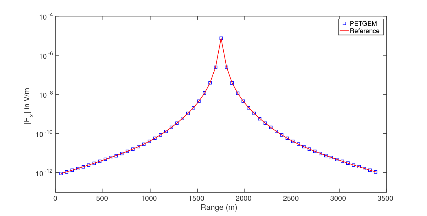
Figure 7.9. Total electric field comparative for x-component between PETGEM V1.0 and DIPOLE1D.¶

Example 2: Use of high-order Nédélec elements ¶

In order to show the potential of high-order Nédélec elements, here is considered the same model of previous example. In this case, the Nédélec element order is p=2 (second order).

Meshing ¶

As in previous example, the mesh is composed by four conductivity materials. The resulting Gmsh script can be found in Download section. It is worth to mention that the use a Nédélec element order p=2 helps to reduce the number of tetrahedral elements to achieved a certain error level.

Parameters file for PETGEM ¶

The parameters file used for this example follows:

###############################################################################
# PETGEM parameters file
###############################################################################
# Model parameters
model:
  mode: csem    # Modeling mode: csem or mt
  csem:
    sigma:
      #file: 'my_file.h5'                # Conductivity model file
      horizontal: [1., 0.01, 1., 3.3333]  # Horizontal conductivity
      vertical: [1., 0.01, 1., 3.3333]    # Vertical conductivity
    source:
      frequency: 2.                     # Frequency (Hz)
      position: [1750., 1750., -975.]   # Source position (xyz)
      azimuth: 0.                       # Source rotation in xy plane (in degrees)
      dip: 0.                           # Source rotation in xz plane (in degrees)
      current: 1.                       # Source current (Am)
      length: 1.                        # Source length  (m)
  mt:
    sigma:
      file: 'my_file.h5'                # Conductivity model file
      #horizontal: [1.e-10, 0.01]       # Horizontal conductivity
      #vertical: [1.e-10, 0.01]         # Vertical conductivity
    frequency: 4.                      # Frequency (Hz)
    polarization: 'xy'                 # Polarization mode for mt (xyz)

  # Common parameters for all models
  mesh: examples/case_2/DIPOLE1D.msh   # Mesh file (gmsh format v2)
  receivers: examples/case_2/receiver_pos.h5 # Receiver positions file (xyz)

# Execution parameters
run:
  nord: 2       # Vector basis order (1,2,3,4,5,6)
  cuda: False   # Cuda support (True or False)

# Output parameters
output:
  vtk: True                               # Postprocess vtk file (EM fields, conductivity)
  directory: examples/case_2/out           # Directory for output (results)
  directory_scratch: examples/case_2/tmp   # Directory for temporal files

Running PETGEM ¶

To run the simulation, the following command should be run in the top-level directory of the PETGEM source tree:

$ mpirun -n 48 python3 kernel.py -options_file case2/petsc.opts case2/params.yaml

kernel.py solves the problem as follows:

Problem initialization
Preprocessing data
Import files
Parallel assembly system
Parallel solution system
Post-processing of electric responses

and outputs the solution to the output path (case2/out). The output files will be in hdf5 format.

Nédélec order comparison ¶

Figure 7.10 shows a comparison of the x-component of total electric field between p=1 and p=2 against the quasi-analytical solution obtained with the DIPOLE1D tool. The total electric field in Figure 7.10 was calculated using a mesh with $\approx2$ millions of DOFs for p=1 and a mesh with $\approx600$ thousands of DOFs.

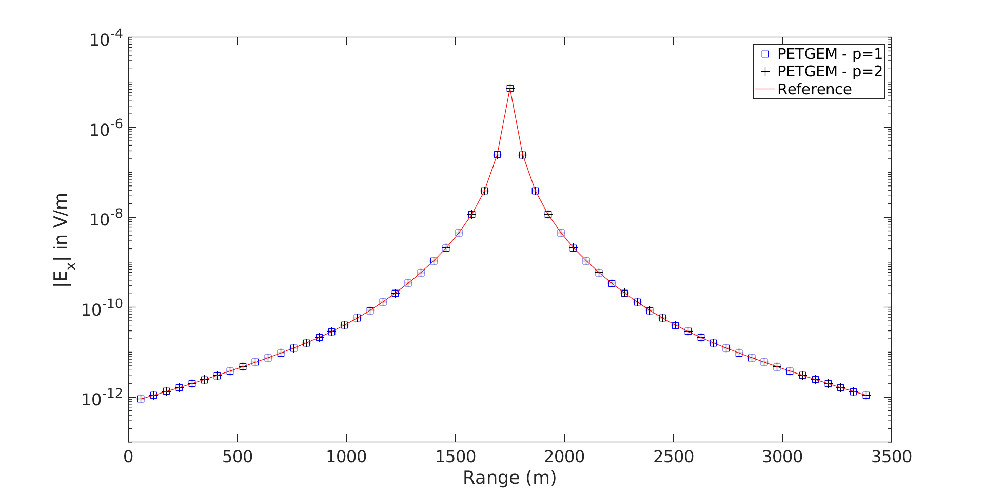
Figure 7.10. Nédélec order comparative within PETGEM V1.0¶

Example 3: Use of PETSc solvers ¶

In PETGEM, options for PETSc solvers/preconditioners are accessible via the petsc.opts file. Here is presented a short list of relevant configuration options for the solution of the problem under consideration.

Direct solver by MUMPs via PETSc interface

# Solver options for PETSc
-pc_type lu
-pc_factor_mat_solver_package mumps

Generalized minimal residual (GMRES) solver with a successive over-relaxation method (SOR) as preconditioner. Further, these options prints useful information: True residual norm, the preconditioned residual norm at each iteration and reason a iterative method was said to have converged or diverged.
```
# Solver options for PETSc
-ksp_type gmres
-pc_type sor
-ksp_rtol 1e-8
-ksp_monitor_true_residual
-ksp_converged_reason
```
Generalized minimal residual (GMRES) solver with a geometric algebraic multigrid method (GAMG) as preconditioner.
```
# Solver options for PETSc
-ksp_type gmres
-pc_type gamg
-ksp_rtol 1e-8
```
Generalized minimal residual (GMRES) solver with an additive Schwarz method (ASM) as preconditioner.
```
# Solver options for PETSc
-ksp_type gmres
-pc_type asm
-sub_pc_type lu
-ksp_rtol 1e-8
```
Generalized minimal residual (GMRES) solver with a Jacobi method as preconditioner.
```
# Solver options for PETSc
-ksp_type gmres
-pc_type bjacobi
-ksp_rtol 1e-8
```
Transpose free quasi-minimal residual (TFQMR) solver with a successive over-relaxation method (SOR) as preconditioner.
```
# Solver options for PETSc
-ksp_type tfqmr
-pc_type sor
-ksp_rtol 1e-8
```

Previous configuration are based on most used in the literature.

MT example ¶

This section includes a step-by-step walk-through of the process to solve a simple 3D MT survey. The typical process to solve a problem using PETGEM is followed: a model is meshed, PETGEM input files are preprocessed and modeled by using kernel.py script to solve the modelling and finally the results of the simulation are visualised.

All necessary data to reproduce the following examples are available in the Download section.

Example 4: 3D trapezoidal hill model ¶

Model ¶

In order to explain the 3D MT modelling using PETGEM, here is considered a 3D trapezoidal hill model. This test case is a homogeneous half-space model with 1/100 $S/m$ as host resistivity and 1e-9 $S/m$ as the free-space resistivity. The trapezoidal hill, centered at the computational domain, has a height of 0.45km with a hill-top square of 0.45km X 0.45km, and a hill-bottom square of 2km X 2km. A cross-section view of the model under consideration is depicted in Figure 7.11. By using the horizontal components of the EM fields at 2Hz, the apparent resistivities are computed. 41 sites at 0km and along the x-axis are arranged equidistant spacing over the interval x=[-2:2]km. Further, the Nédélec element order is p=2 (second order).

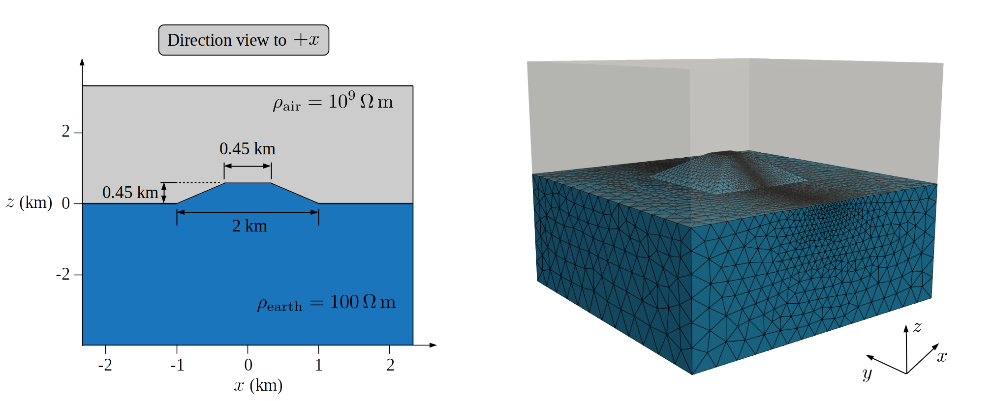
Figure 7.11. Cross-section view of the 3D trapezoidal hill model (left-panel) with its resulting computational unstructured and hp-adapted mesh for p = 2 (right-panel).¶

Parameters file for PETGEM ¶

The parameters file used for this example follows:

###############################################################################
# PETGEM parameters file
###############################################################################
# Model parameters
model:
  mode: mt    # Modeling mode: csem or mt
  mt:
    sigma:
      #file: 'my_file.h5'                # Conductivity model file
      horizontal: [1.e-10, 0.01]       # Horizontal conductivity
      vertical: [1.e-10, 0.01]         # Vertical conductivity
    frequency: 2.                      # Frequency (Hz)
    polarization: 'xy'                 # Polarization mode for mt (xyz)

  # Common parameters for all models
  mesh: examples/case_4/mesh_trapezoidal.msh   # Mesh file (gmsh format v2)
  receivers: examples/case_4/receivers.h5 # Receiver positions file (xyz)

# Execution parameters
run:
  nord: 2       # Vector basis order (1,2,3,4,5,6)
  cuda: False   # Cuda support (True or False)

# Output parameters
output:
  vtk: False                               # Postprocess vtk file (EM fields, conductivity)
  directory: examples/case_4/out           # Directory for output (results)
  directory_scratch: examples/case_4/tmp   # Directory for temporal files

Note that you may wish to change the location of the input files to somewhere on your drive. The solver options have been configured in the petsc.opts file as follows:

# Solver options for
-pc_type lu
-pc_factor_mat_solver_package mumps

That’s it, we are now ready to solve the modelling.

Running PETGEM ¶

To run the simulation, the following command should be run in the top-level directory of the PETGEM source tree:

$ mpirun -n 16 python3 kernel.py -options_file case4/petsc.opts case4/params.yaml

kernel.py solves the problem as follows:

Problem initialization
Preprocessing data
Import files
Parallel assembly system (twice, 1 for each polarization mode)
Parallel solution system (twice, 1 for each polarization mode)
Post-processing of electric responses, apparent resistivities and phases

and outputs the solution to the output path (case4/out/). The output file will be in hdf5 format.

PETGEM post-processing ¶

Once a solution of a 3D MT survey has been obtained, it should be post-processed by using a visualization program. PETGEM does not do the visualization by itself, but it generates output file (hdf5) with the electric responses (apparent resistivities and phases) and receivers positions. It also gives timing values in order to evaluate the performance.

The electric fields responses can be handled freely and plotted. The dimension of the array is determined by the number of receivers in the modelling (41 in this example). Figure 7.12 shows a comparison of the obtained apparent resistivity and phase.

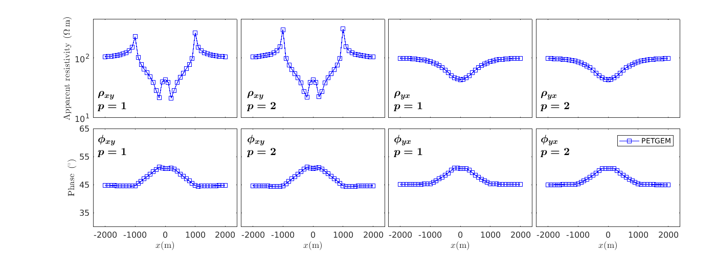
Apparent resistivities (left-panel) and phases (right-panel) for the 3D trapezoidal hill model. The PETGEM solutions were calculated with p = 2.

Figure 7.12. Apparent resistivities (left-panel) and phases (right-panel) for the 3D trapezoidal hill model. The PETGEM solutions were calculated with p = 2.¶

Code documentation ¶

Following sub-sections are dedicated to code documentation of PETGEM.

HEFEM scripts ¶

Solver ¶

solver.py

Parallel ¶

parallel.py

Post-processing ¶

preprocessing.py

Previous topic

Next topic

Manual¶

How generate documentation ¶

Coding style ¶

PETGEM design ¶

PETGEM directory structure ¶

Running a simulation ¶

Mesh formats ¶

Available solvers ¶

Simulations in parallel ¶

Visualization of results ¶

CSEM example ¶

Example 1: Canonical model of an off-shore hydrocarbon reservoir ¶

Model ¶

Meshing ¶

Parameters file for PETGEM ¶

Running PETGEM ¶

PETGEM post-processing ¶

Example 2: Use of high-order Nédélec elements ¶

Meshing ¶

Parameters file for PETGEM ¶

Running PETGEM ¶

Nédélec order comparison ¶

Example 3: Use of PETSc solvers ¶

MT example ¶

Example 4: 3D trapezoidal hill model ¶

Model ¶

Parameters file for PETGEM ¶

Running PETGEM ¶

PETGEM post-processing ¶

Code documentation ¶

kernel ¶

Common scripts ¶

Pre-processing ¶

Mesh scripts ¶

HEFEM scripts ¶

Solver ¶

Parallel ¶

Post-processing ¶